PULSE: probabilistic simulation of intensive-care trajectories
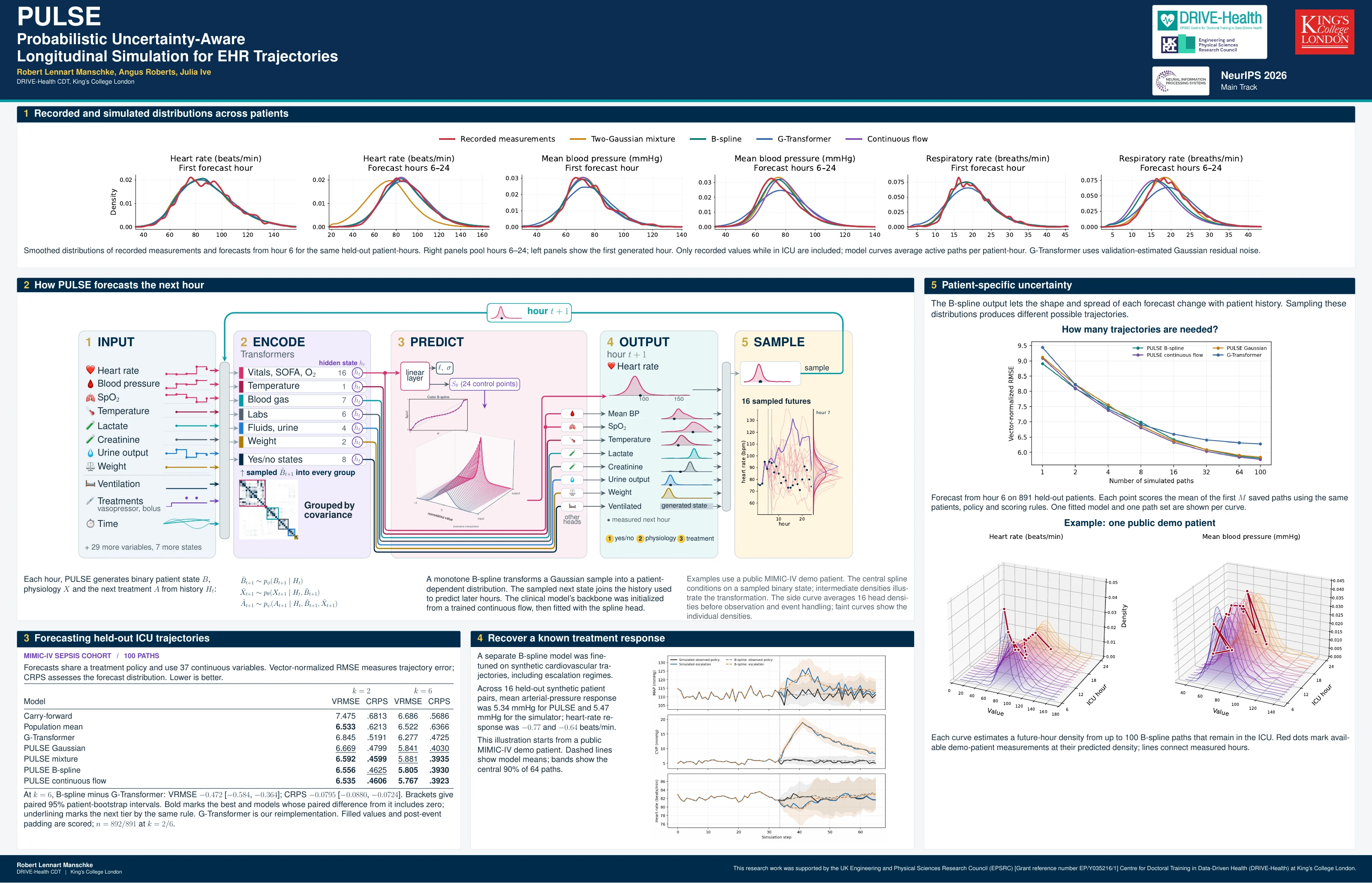
PULSE generates possible trajectories for patients in intensive care. It learns how physiology and uncertainty change with a patient’s history and treatments, predicting a probability distribution for each continuous measurement.
Sampling from these distributions produces multivariable patient records. Their shape and spread can change as a simulated patient’s condition evolves, allowing the model to represent patient-dependent variability.
Loading forecast distributions…
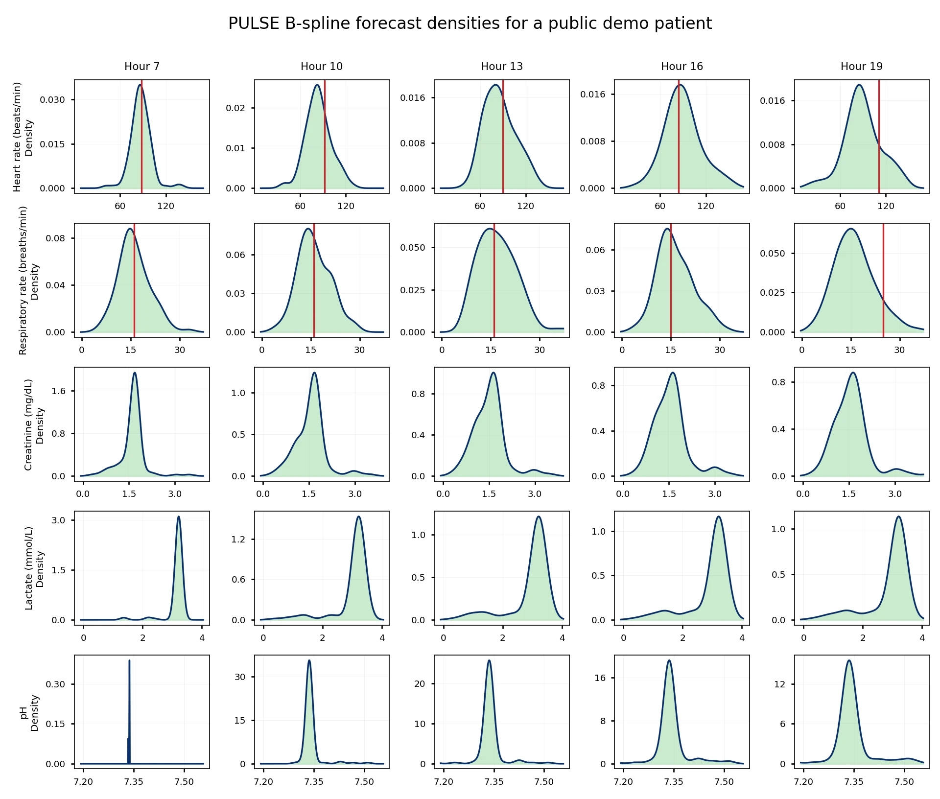
B-spline forecast densities for a patient in the public MIMIC-IV demo database. The red line follows recorded measurements. Drag the figure to rotate it, or scroll over it to zoom.
Why model distributions?
Predicting a patient’s future involves uncertainty about both the values that will be observed and how variable those values may be. Two patients with the same expected heart rate can have different ranges of plausible outcomes. A simulator should be able to represent those differences and update them as new observations, treatments and events become part of the patient’s history.
Generating realistic synthetic records also requires accuracy at two levels. Individual trajectories should reflect the patient’s condition, while distributions across many simulated patients should resemble those in recorded data. Agreement at one level does not establish agreement at the other, so we examine patient-level forecasts and population-level distributions separately.
Existing sequential simulators provide a foundation for this work. PULSE extends that approach by learning continuous distributions whose shape and spread depend on patient state. This changing variability is called heteroskedasticity. We also want simulated trajectories to respond to changes in treatment. A controlled synthetic benchmark, where treatment effects are known, lets us examine that behaviour before considering clinical applications.
Patient-level forecasts
The example below follows a patient from the public MIMIC-IV demo database. PULSE reads the available history and generates possible subsequent trajectories. Select a measurement and move through forecast hours to compare the distribution at each hour with the recorded value. The trajectory view shows how uncertainty accumulates across generated histories.
Possible trajectories
Forecast begins at hour 6Distribution at the selected hour
Hour 13Saved forecasts from one fitted B-spline model, using 100 paths and a shared treatment policy. Curves estimate densities from active paths; the shaded interval describes their spread. A single patient illustrates model behaviour. Aggregate evaluation follows below.
How PULSE generates trajectories
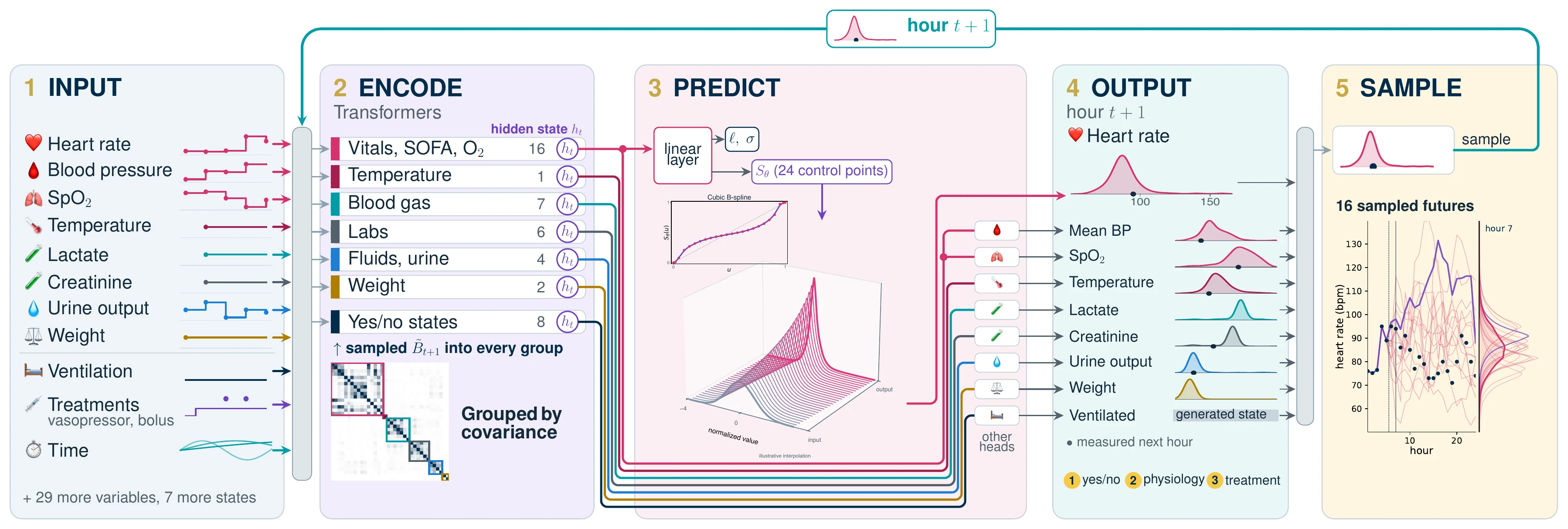
PULSE represents patient history using observed values, observation masks, treatments and static patient information. Variables whose changes are correlated in the training data share an encoder, while each variable retains its own output distribution. Sharing an encoder lets related measurements reuse the same computation over patient history.
The model predicts binary patient state before continuous physiology. Each continuous head then predicts a location, a scale and a monotone B-spline transformation conditioned on history and the next binary state. A sampled patient state is appended to history, and a separate treatment policy supplies actions for subsequent steps. Repeating this process generates a possible trajectory.
The B-spline output distribution
A B-spline is a smooth curve built from simple polynomial pieces. PULSE learns an increasing transformation conditioned on patient history. Its bends can change the skew, tails and spread of a distribution.
Slide from input to output to reveal one fitted heart-rate transformation. Intermediate stages interpolate between the two maps for illustration.
z ∼ 𝒩(0, 1) → μ(h) + σ(h) f(z; h)
Here h represents patient history; the location, scale and transform all depend on it.
Normal input and transformed density
How do conditional distributions combine across paths?
Every generated history conditions its own next-step distribution. Averaging these conditional densities represents uncertainty across possible histories as well as uncertainty in each next value.
This example averages 16 saved B-spline head densities at hour 7 for a public-demo patient. Faint curves show normalized components; the bold curve is their equal-weight average.
How does PULSE handle incomplete observations?
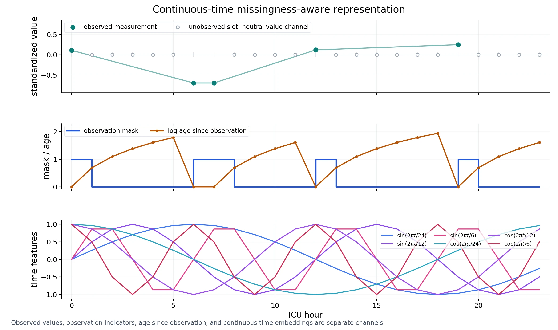
Observation masks identify which entries were measured. Event-time variants also expose elapsed time and measurement age, so a missing entry and a newly observed value remain distinguishable. These variants are evaluated separately in the paper.
The headline evaluation scores forward-filled and post-event padded targets. Its numerical comparison therefore answers a different question from the recorded-measurement distribution plots below.
Distributions across patients
These figures compare recorded measurements with values generated for the same held-out patients. The first panel shows the first forecast hour; the second pools hours 6–24. Comparing the panels reveals how each model’s population distribution changes as generated values feed back into its history. Select a measurement and use the model labels to choose which curves are visible.
First forecast hour
Hour 6Across forecast hours
Hours 6–24Predictive performance on MIMIC-IV
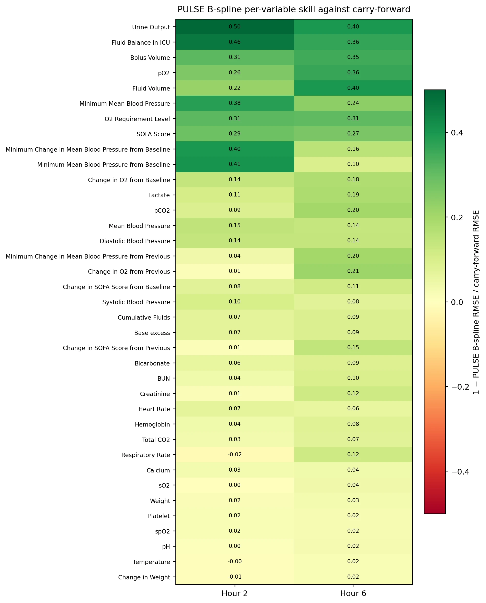
We compare separately fitted models on the same held-out MIMIC-IV sepsis patients, using a shared treatment policy, 100 sampled paths and scoring over 37 variables. Vector root mean squared error (VRMSE) measures error in the average forecast. Continuous ranked probability score (CRPS) evaluates the full predictive distribution, rewarding forecasts that concentrate probability around the observed outcome.
When forecasting from hour 6, the B-spline model has 7.5% lower VRMSE and 16.8% lower CRPS than our G-Transformer reimplementation. The paired patient-bootstrap intervals for both differences exclude zero. Both scores also improve when forecasting from hour 2. The table gives the numerical results and confidence intervals for each comparison.
| Model | Vector RMSE ↓Average-forecast error | CRPS ↓Distributional score | 90% coverageTarget: 0.90 |
|---|
Brackets give 95% patient-bootstrap intervals. Bold marks the best value and values whose paired interval against it includes zero. Underlining marks the next tier by the same rule. This expresses a lack of detected difference; it does not establish equivalence. Coverage tiers use proximity to 0.90.
What do these scores measure?
Vector root mean squared error (VRMSE) measures error after averaging sampled trajectories. Continuous ranked probability score (CRPS) evaluates the full forecast distribution; lower values are better. Coverage measures how often a central 90% forecast interval contains the target, with 0.90 as its reference.
The main comparison uses forward-filled and post-event padded targets. G-Transformer is our reimplementation. Each row uses one fitted model; patient-bootstrap intervals describe variation across patients. Training initialization and model settings are documented in the paper and code repository.
Convergence as more trajectories are sampled
Averaging more sampled trajectories stabilizes the mean forecast. These curves rescore increasing subsets of the same 100 saved paths.
At hour 6, 32 B-spline paths yield VRMSE 6.086, compared with 6.277 for 100 G-Transformer paths. This is a score comparison; total compute also depends on architecture, hardware and implementation.
Subset curves show sample convergence for these fits. They do not measure timing or independent reruns.
Treatment responses in a synthetic benchmark
A cardiovascular benchmark inspired by CVSim provides a setting in which treatment responses are known. We fit a separate B-spline model to synthetic trajectories, including treatment-escalation regimes, and compare its predictions with the simulator under two treatment histories starting from the same patient state.
This illustration starts from public-demo patient information. Solid lines show the synthetic simulator; dashed lines show model means, with central 90% ranges from 64 paths per treatment policy.
Treatment changes at simulation step 34. Shading shows variation across generated paths from a single fitted model.
Across 16 held-out synthetic patient pairs, the mean arterial-pressure response was 5.34 mmHg for PULSE and 5.47 mmHg for the simulator, using 32 paths per policy. Recovering known synthetic responses is one step toward evaluating treatment-sensitive simulation. Clinical treatment effects require additional causal and clinical validation.
Research directions
We hope that patient-dependent distributions can support more realistic synthetic data and make uncertainty easier to inspect. Continuous probabilistic outputs offer a direct way to learn uncertainty in measurements expressed on continuous scales.
Longer term, we want to help researchers build systems that explain possible trajectories and explore treatment choices with evidence. Clinical validation, causal identification and evaluation across populations remain essential work before such systems can inform patient care.
Paper and related materials
Paper
B-spline camera-ready manuscript, methods and appendices.
Poster
A visual tour of the architecture, evidence and examples.
Presentation
An animated walkthrough of the poster and its figures.
Code on GitHub
Build cohorts, fit models, generate trajectories and score forecasts.
More figures from the paper
Cite PULSE
@inproceedings{manschke2026pulse,
  title = {PULSE: Probabilistic Uncertainty-Aware Longitudinal Simulation for EHR Trajectories},
  author = {Manschke, Robert Lennart and Roberts, Angus and Ive, Julia},
  booktitle = {Advances in Neural Information Processing Systems},
  year = {2026}
}
Data and reproducibility
Individual examples on this page use the public MIMIC-IV demo database or synthetic trajectories. Clinical comparisons are cohort aggregates. The code describes training and evaluation with credentialed-access MIMIC-IV data. Trained weights are not included. Figure and data provenance ↗